Going steady (state) with Markov processes

After the finite midterm, you may have been confused and annoyed when the class seemed to abruptly shift from probabilities and permutations to matrices and systems of equations. They seem to have nothing to do with each other!

Well, today is your lucky day. Probability theory and matrices have finally met, fallen in love, and had a beautiful baby named Markov.

Let me explain. Markov processes are widely used in economics, chemistry, biology and just about every other field to model systems that can be in one or more states with certain probabilities. These probabilities change over time.

For example, we might want model the probability of whether or not Amazon.com turns a profit each quarter. So, Amazon.com (the system) can be in two possible states at the end of each quarter: either they turn a profit, or they don't. Their chance of turning a profit this quarter depends on whether or not they turned a profit last quarter. For example, if they profited last quarter, they might be more likely to profit again this quarter.

The crucial assumptions for describing Amazon.com's performance as a Markov process are:

1. We can divide time up into discrete units (in this case, quarters), and;
2. Their chances of profiting this quarter depend only on how they did last quarter.

There are continuous Markov processes as well, where we don't have to divide time into quarters, or days, but we won't worry about that case for now.

So, what's the point? Well, we can use Markov processes to answer questions like "what are the chances that Amazon will profit 6 quarters from now?", or "what are the long-run chances that Amazon will profit in a given quarter?" This last question is particularly important, and is referred to as a steady state analysis of the process.

To practice answering some of these questions, let's take an example:

Example: Your attendance in your finite math class can be modeled as a Markov process. When you go to class, you understand the material well and there is a 90% chance that you will go to the next class. However when you skip class, you become discouraged and so there is only a 60% chance that you'll go to the next class.

Suppose that you attend the first day of class. What are your chances of attending the next class? What about the next few classes after that? What are your chances of attending class in the long run?

Ok, so we have two states: attend and absent. For each of these states, there is a chance that we'll be in that same state for the next class, but there is also a chance that we'll switch to the other state. Thus, we have four probabilities:

1.\(P(attend \to attend) = 0.9\) 2.\(P(attend \to absent) = 0.1\) 3.\(P(absent \to attend) = 0.6\) 4.\(P(absent \to absent) = 0.4\)

It turns out that we can model these four probabilities in a matrix:

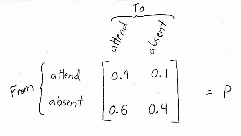
Notice that the rows represent the state we're going from, and the columns represent the state we're going to. Also, notice that the probabilities in each row add up to 1. This is because each row represents the probabilities of all the possible states that we could end up in for the next "time step" (class).

This matrix, which I've named \(P\), is called the transition matrix. It completely describes the probabilities of transitioning from any one state to any other state at each time step.

But how do we represent the probabilities of actually being in a particular state at a specific point in time? To do this, we use a state vector. In this example, we know that we're in the state "attend" for the first class. So, our probability of attending the first class is 1 and our probability of being absent is 0. We represent this as a horizontal vector (you'll see why in a minute):

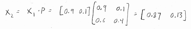
So, to answer the question "what is the probability of attending the next class?", we just need to multiply our current state vector by the transition matrix to get the next state vector:

Well, that seems to make sense. There is a 90% chance that we'll attend the next class, and a 10% chance that we won't - this is exactly what the problem told us in the first place!

What about the next class after that? Well, we know the state vector \(X_1\), so we can use it to compute \(X_2\) the same way that we used \(X_0\) to compute \(X_1\):

And so forth:

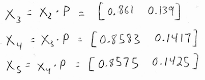
If you keep doing this forever, you'll notice that the probability of going to class is getting smaller, but it doesn't seem to be approaching zero. In fact, it seems to be approaching a very specific number, somewhere around 0.857...

So, what's going on here? In the long run, the system approaches its steady state. The steady state vector is a state vector that doesn't change from one time step to the next. You could think of it in terms of the stock market: from day to day or year to year the stock market might be up or down, but in the long run it grows at a steady 10%.

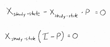
This notion of "not changing from one time step to the next" is actually what lets us calculate the steady state vector:

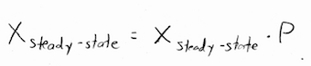
In other words, the steady-state vector is the vector that, when we multiply it by \(P\), we get the same exact vector back. Now, of course we could multiply zero by \(P\) and get zero back. But, this would not be a state vector, because state vectors are probabilities, and probabilities need to add to 1. It turns out that there is another solution. With a little algebra:

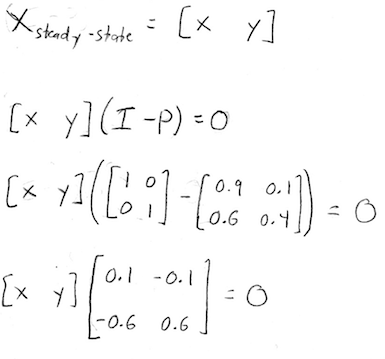
\(I\) is the identity matrix, in our case the 2x2 identity matrix. If we write our steady-state vector out with the two unknown probabilities \(x\) and \(y\), and we compute \(I-P\), we get:

Let's write this out in equation form, just to get a better sense of what we're trying to solve:

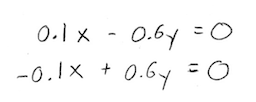
Great, we're ready to solve this, right? Not so fast. What do you notice about these two equations?

Yup, you got it. They're the same equation. The bottom one is just the top equation multiplied by -1. So, we really only have one equation. And with one equation and two unknowns, we'd have an infinite number of solutions.

But clearly, there is a specific steady state vector for our system. So, we're going to need to find another equation somewhere. How can we do this?

Well, remember that \(x\) and \(y\) represent probabilities - the probabilities of the only two possible events (either we attend class, or we are absent)! This means that they need to add to 1:

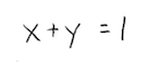
Ahh, that's better. So, putting this equation together with one of the equations from before, we can write:

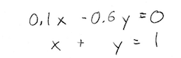
Or in matrix form:

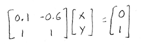
Now that's something we know how to solve! Using row-reduction, of course:

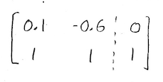
Multiply everything by 10 to make our arithmetic easier:

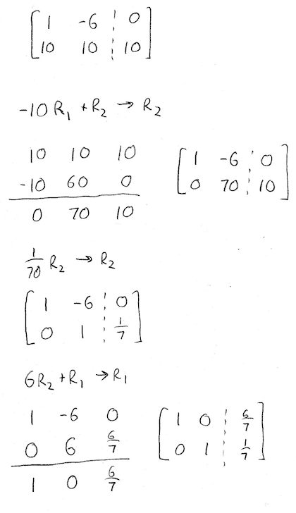
And there we have it, our steady-state vector is:

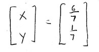
So in the long run, we'll attend class with probability \(\frac{6}{7}\), and skip with probability \(\frac{1}{7}\). Notice that \(\frac{6}{7}\approx 0.85714...\), which is close to the values we were seeing earlier.

Ok, good luck and see you next time!