When to use INDEX-MATCH, VLOOKUP, or HLOOKUP

Today's post is courtesy of our awesome K201 tutor Dalia, who wants you to get comfortable with some of Excel's more common lookup and indexing functions. This is one of the hardest parts of Excel for most people, and where students tend to get stuck in the class.

One of the more powerful features of Excel is the ability to automatically cross-reference a table of values based on some input value(s). For example, you might have a spreadsheet that computes your company's total revenue from each customer, but to do that it must look up the hourly rate and total number of billed hours for each customer from another spreadsheet. When used like this, spreadsheets can almost (but not quite) be used like the relational databases you studied in the first half of K201.

The most common functions you'll use for cross-referencing in Excel are:

• VLOOKUP and HLOOKUP
• MATCH
• INDEX

Both VLOOKUP and HLOOKUPs are used in the same way, so from now on we'll just refer to them collectively as the *LOOKUP functions.

When tackling a question in K201 that requires you to do some kind of cross-referencing, you first need to figure out which function(s) you need to use. *LOOKUP functions are simpler, but a combination of MATCH and INDEX is much more powerful. Actually, anything you can do with a *LOOKUP can be done with a combination of MATCH and INDEX instead!

To decide if you can use a *LOOKUP, or if you need to use INDEX and MATCH, you need to look at two things: the input (the information you're using to do the lookup), and the output (the information you're trying to get). When you're trying to look up a value based on a single input, you may be able to use a *LOOKUP function. If you're explicitly asked to find the location of a single input, or to look something up using two or more pieces of information, you'll need to use the MATCH and/or INDEX functions instead.

Performing a lookup based on a single input

Take the following example:

Write a formula that returns the Product Number based on the Product Name.

For this example, we have one input: the Product Name. Next, ask yourself "does my formula need to return the value, or the location (row or column number) as output?" In this example, you are looking for a value: the Product Number. When we have only a single input, and we're looking for a value output, we can use a VLOOKUP or HLOOKUP (depending on how the data is displayed).

The syntax for *LOOKUP functions is as follows:

=*LOOKUP(lookup_value, table_array, row(or column)_num, TRUE or FALSE)

The lookup_value is the input value on which you want to perform the lookup. The table_array is the range in which the information is found: do NOT include column headings as part of this range. In order for a *LOOKUP to work correctly, the lookup_value must be in the first row or column of the table_array. This means that you need to choose a range for table_array so that your input is in the first row or column.

The row_num or column_num is the relative position of the row or column where your output data can be found. For our example, we want the row or column number containing the table's Product Numbers. It is important to note that row_num and column_num are not necessarily the same as your spreadsheet's row and column references! Rather, they are relative to the first row or column of the range specified in table_array. Thus the row or column containing the actual lookup_value is always 1 (the first row or column of the table_array). The next row or column in your range is 2, and so forth.

If you set the last parameter of your lookup function to TRUE, you are saying that your lookup_value is approximate. TRUE is mostly used for numbers that belong to number ranges (but not exclusively). FALSE indicated that the lookup_value is an exact match.

Let's look at another example:

Write a formula that finds the row number of a certain product based on the Product Name.

Again, we have a single input - the Product Name. However in this example, we're looking for the location of our input value. That means that this example is looking for a MATCH.

Generally speaking, MATCH isn't often used by itself in the real world. Usually we use MATCH together with an INDEX function. However, we'll talk about INDEX later - for this example all we need is MATCH.

The syntax for MATCH is:

=MATCH(lookup_value, lookup_array, match_type)

The lookup_value for MATCH is essentially the same thing as the lookup_value of a *LOOKUP (except you do not have to worry if the input value is in the first row/column of the table_array, because a MATCH uses a lookup_array.)

The lookup_array is the cell range to search for your lookup_value. Make sure that you select only ONE row or column for your lookup_array - not the whole table.

Finally, the match_type is similar to the *LOOKUP's last parameter (the one that can be TRUE or FALSE). The difference is that MATCH functions use a numeric value for match_type: -1 means "less than," 0 means "exact match," and 1 means "greater than." For our example, we would use 0.

Performing a lookup based on two inputs

Suppose we have the following problem:

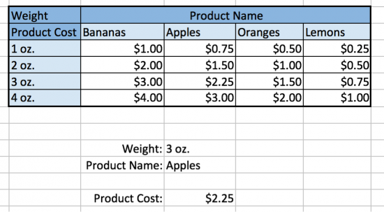
For the table below, write a formula to find the Product Cost based on the Product Name and the Weight. Then, use this formula to determine how much 3 oz. of Apples will cost.

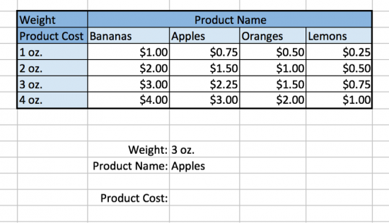
From this table it is obvious to see that 3 oz. of Apples cost $2.25, but what if you wanted a way to quickly look up the cost from thousands of rows of data? Or, what if you wanted to use the cost of each product in another formula or spreadsheet? This is why we use an INDEX function.

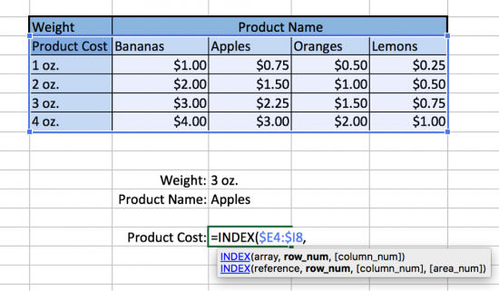
=INDEX(array, Vertical MATCH, horizontal MATCH)

First let's define array – the table that where the information is found. When using INDEX, I highly recommend including the header row and column (the ones that contain the product names and weights). This is so that, if you select the entire row or column in your MATCH formulas, the relative positions found will line up with the relative positions expected by INDEX. Make sure to lock/anchor your array, because we do not want this to ever change.

Our column headings are the various weights and the various types of products.

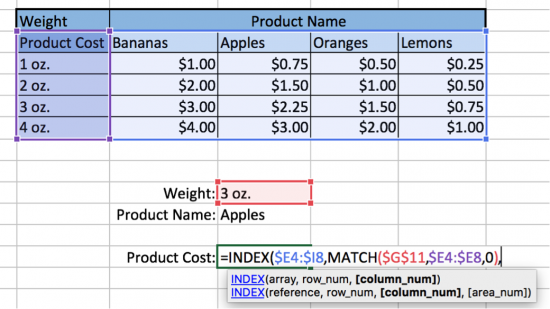
Next, we start our vertical MATCH.

Recall that the syntax is =MATCH(lookup_value, lookup_array, match_type).

Our lookup_value in this example is the weight. We pick a cell to use for our input weight, reference it in our formula, and anchor it using the F4 key.

Our lookup_array is where we will find the weight. Make sure that you stay inside the range you specified for array, and include everything in that column. Once it is selected, we will anchor it so that it never changes.

Finally, our match_type is 0 because we want an exact match against the product weight - for example "3 oz."

Finally, we we start our horizontal MATCH.

Our lookup_value in this example is the product name. We pick another cell to use for our input product name, reference it in our formula, and again anchor it using the F4 key.

Our lookup_array is the range to search for the product name. Make sure that you stay inside the range you specified for array, and include everything in that row. Once it is selected, we will anchor it so that it never changes.

Finally, our match_type is 0 because we want an exact match against the product name - for example "Apples."

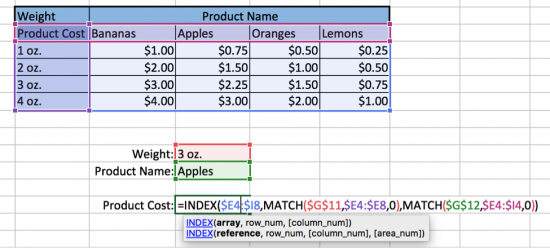
If all the above steps are done correctly, you will get the answer of $2.25.

Notice that we can now fill in any combination of values in our Product Name and Weight input cells, and our formula will find the corresponding Product Cost. We could even link the output of another formula to these input cells (for example, looking up the Product Name from a customer invoice), for even more sophisticated business situations.

Wow, amazing! Your K201 GPs don't stand a chance.